EngineeringOctober 8, 2026

Pushingthelimitsofsatellitecontactplanningwithphysics-informedforecasting

How time-varying link forecasts change throughput, failed passes, and ground-station selection.

By Laith Altarabishi

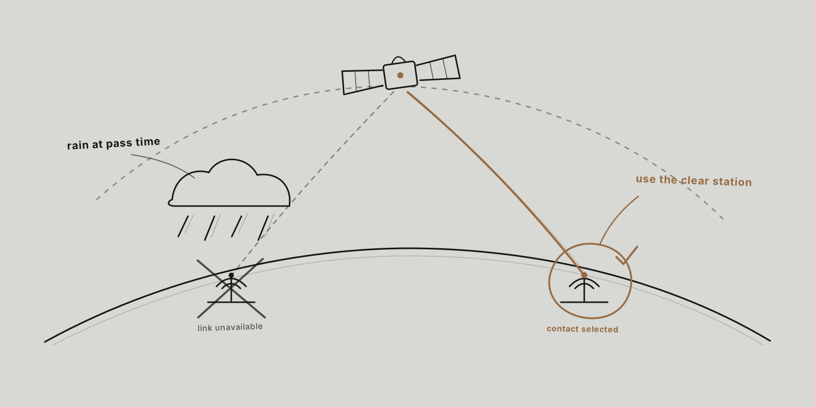
Hand-drawn contact plan routing a satellite pass away from rain toward a clear ground station

Conventional satellite mission operations involve a tremendous amount of human-in-the-loop monitoring and reactive decision-making¹, and even highly automated constellation operators say human-centred operations do not scale to hundreds of satellites². We believe this is a key point of failure as satellite networks scale and grow in complexity.

About 11,000 active satellites orbit Earth today³, but regulatory filings already propose far more, including about 7,700 satellites now authorized for Amazon's LEO system⁴ and up to one million in a single SpaceX application⁵. In a future with this many assets in space, a classical networking question becomes central: how to best schedule contacts. A contact is a time-constrained opportunity to transmit data between two nodes in a satellite network topology. Scheduling those contacts is already computationally hard: satellite range scheduling is NP-complete⁶, and contact-plan design is a combinatorial problem whose complexity grows exponentially with the size of the network⁷.

Today, contact plans are mostly computed ahead of time from orbit propagation and link models, with weather margins sized from long-term statistics, and then reserved with ground providers^8,9. The physics behind them is modelled with various degrees of fidelity, with the fundamental limitation being that the problem is inherently dynamic and time-varying: a plan that assumes contacts are predictable has no room to adapt when a prediction is wrong⁷.

The physics of orbital mechanics, atmospheric conditions, and link budgets change continuously, and any static snapshot of the problem misses the rich temporal structure that determines when and how data can actually be moved through the network. With the growing trend of ground station and satellite operators moving into higher-frequency spectrum and optical wavelengths, atmospheric attenuation grows and link availability depends more and more on the weather^10,11,12.

Forecasting the link budget, rather than sizing it from long-term statistics, moves more data for every booked minute of antenna time and loses fewer passes. In this article, we show this for two high-frequency bands, Ka and optical. For Ka links, which degrade gradually with rain, a forecast tells us how much margin we actually need on a given pass. For optical links, which a single cloud can block completely, it tells us which station to book.

A quick primer into RF physics and link budgets

The link budget

The link budget is like an accounting sheet for a communication link: it tells us how much signal power we have at the transmitter, how much is lost to free-space path loss, atmospheric attenuation, and other impairments, and how much power ultimately arrives at the receiver.

P_Rx = P_Tx + G_Tx − L_FS − L_ATM − L_other + G_Rx dBW

Figure 1 is that accounting sheet for an illustrative Ka-band downlink. Move the rain slider: the atmosphere is the one term that changes from minute to minute, and the received power and the signal above noise move with it.

This link budget tells us the theoretical signal power received, and, after converting it from dB to linear units, we can compare it with the receiver's thermal noise power. That noise term decomposes into three physical quantities:

N = k · T_sys · B

k is the Boltzmann constant, 1.380649 × 10⁻²³ J/K;T_sys is system noise temperature in kelvin; andB is receiver bandwidth in hertz. Their product isN, the noise power in watts. The signal-to-noise ratio is therefore:

SNR = P_RxN = P_Rxk · T_sys · B

With the SNR estimate, we can compute the Shannon capacity, which gives us the theoretical maximum data rate that can be reliably transmitted over the channel¹³:

C = B log₂(1 + SNR) bit/s

From capacity to MODCODs

However, in practice, given the continuous and theoretical nature of Shannon capacity, we work with discrete modulation and coding schemes (MODCODs) that map specific SNR ranges to achievable data rates. Each MODCOD defines a combination of modulation order and code rate, and the system selects the highest-order MODCOD whose required SNR threshold is met under current link conditions. The DVB-S2X standard, for example, defines a set of MODCODs, each with a specified spectral efficiency and a required E_s/N₀ threshold¹⁴.

Figure 2 shows that staircase under the Shannon curve. Drag the fade bracket left from the clear-sky point: the operating point drops one rung at a time, then falls off the bottom.

With this, we can now understand how RF links behave under varying atmospheric conditions. The key insight is that L_ATM is not a constant: rain, clouds, and scintillation introduce time-varying losses that can push the link below a given MODCOD threshold, forcing the system to fall back to a lower-order MODCOD or, in the worst case, lose the link entirely until conditions improve.

Choosing the MODCOD: CCM, VCM and ACM

Links typically run one of three policies for choosing the MODCOD: CCM (Constant Coding and Modulation), where one MODCOD is used for the whole pass; VCM (Variable Coding and Modulation), where the MODCOD schedule is pre-determined and shipped as a plan prior to a contact, typically as a function of elevation angle¹⁵; and ACM (Adaptive Coding and Modulation), where the MODCOD is adapted in real time based on channel conditions that the receiver reports back over a return link¹⁶.

Most LEO Earth-observation downlinks run CCM or elevation-scheduled VCM, so the MODCOD is fixed before the pass. ACM is in operational use at Planet on X and Ka band, but it is not yet the norm^17,11.

The choice between VCM and ACM has direct implications for contact planning. VCM offers predictability—the operator knows in advance what spectral efficiency to expect for each portion of the pass, which simplifies both link budgeting and capacity scheduling. ACM, by contrast, trades that predictability for efficiency: it allows the link to exploit favorable conditions and fall back gracefully when the channel degrades. The cost is that the achievable data rate becomes a random variable, which complicates the estimate of how much data can actually be delivered during a scheduled pass.

Figure 3 shows one pass with a rain cell crossing the middle of it. The VCM plan is drawn from the start, because it was fixed before the pass; drag the playhead to see what the link actually carried.

With a 3 dB margin, the plan leaves capacity unused in clear sky and asks for more than the link can carry when the cell passes, so frames are lost. ACM follows the link, but nobody knew in advance how much data it would move.

Why a snapshot is not enough

Now naturally there are some obvious issues with trying to model link budgets directly. One key issue is that each loss term in our link budgeting equation is time-varying, stochastic, and potentially correlated with the others. For example, rain, cloud and scintillation come from the same humid air masses. Measured scintillation grows with rain attenuation¹⁸, and the ITU time-series model builds that coupling in¹⁹. Treating them as independent random variables therefore underestimates the variance of the total loss.

A related issue is how much the current link budget tells us about a contact booked for some time in the future. Even if we have a perfect model of the current channel state, the channel state at the time of the contact may be entirely different, and the further out the contact is scheduled, the more uncertain that prediction becomes.

Figure 4 shows what that looks like on a real afternoon in New Jersey. Everything to the right of the booking line was not yet known when the pass was booked.

The pass was booked at 10:53 on a reading of 0.6 dB. A storm cell arrived about 35 minutes later, and the 11:53 pass delivered nothing.

Rain fades decorrelate within tens of minutes to hours, and radar extrapolation loses skill within a few hours, faster for small storm cells^20,21.

In Figure 5 below, you can drag the booking lead: the weather that will be over the station at the pass is, right now, far upwind. An hour out it is 36 km away, so the latest reading keeps almost no information about it, while a nowcast that follows the storm keeps about half.

Ka and optical

Now if we focus on Ka band and optical links specifically, atmospheric attenuation becomes even more pronounced due to the smaller wavelengths involved. Ka band experiences significantly higher rain attenuation than lower bands like X or C, and optical links, for example at 1550 nm, are affected not just by rain but also by clouds, fog, and atmospheric turbulence.

This is because at Ka band the wavelength, about 1.2 cm at 26 GHz, is only a few times larger than a raindrop, about 0.5–6 mm²², so rain absorbs and scatters the signal strongly. ITU-R P.838 gives about 4 dB/km at 26 GHz in 25 mm/h rain, about 11 times the X-band value²³. For Ka band links this means link quality degrades sharply when the link is operating at or near a MODCOD threshold and a rain cell passes.

For optical links the situation is more binary: water-cloud droplets are comparable to or larger than the 1.55 µm wavelength and attenuate by 100–600 dB/km, so a cloud in the line of sight blocks the link, while thin ice cloud costs 1–15 dB^24,25. A single European optical ground station sees a cloud-free line of sight only about 25–75% of the time, depending on climate²⁵.

Figure 6 sends one rain cell across both links. Watch the timing: the cloud deck cuts the laser well before the rain core reaches the Ka path. Grab the cell to move it yourself.

This distinction has profound implications for contact planning, since it means outage models must capture fundamentally different physical processes depending on the link technology.

Why forecasting matters for contact planning

Beyond just physics, an additional layer of financial and logistical constraints from Ground Station as a Service providers introduces market dynamics: pricing, availability, and priority scheduling all influence which contacts are actually feasible or economical to execute.

For example, AWS Ground Station meters antenna time per minute, rounded up, and a contact stopped after it has started is still billed for its full scheduled length unless a replacement contact on the same station covers the remaining time²⁶. Providers also meter antenna time differently: AWS Ground Station, Leaf Space and Viasat publish per-minute metering^27,28, while KSAT and SSC describe their services on a per-pass basis^29,30. This means that the same nominal contact opportunity can have dramatically different economic value depending on the operator's network and service provider, and those tradeoffs are rarely captured in today's planning tools.

When we add in weather, regulatory constraints, and the fact that satellites themselves are often resource-constrained—power, thermal, and onboard storage^31,32—the contact planning problem becomes exceedingly difficult to model with static heuristics and manual scheduling.

Hence, the need for a fundamentally dynamic, forecasting-first approach. Rather than treating contact planning as a periodic optimization over a fixed snapshot of the network, we argue that the right framing is one of continuous forecasting: predicting, ahead of time, the evolution of link quality, resource availability, and operational constraints so that scheduling decisions can be made proactively rather than reactively.

An illustrative case study

To see what this means in practice, let's take an example ground station and explore how we can choose a single contact. The station is in Secaucus, New Jersey, the site from Figure 4. The link is a Ka-band Earth-observation downlink at 26 GHz with a clear-sky E_s/N₀ of 17 dB, running DVB-S2X. In clear sky it carries about 3.1 GB per minute. Antenna time costs $22 per minute, so a 7-minute pass costs $154. Like most LEO Earth-observation downlinks, the MODCOD is fixed before the pass.

Three planners book the link:

The static planner uses one link budget with a fixed 3 dB weather margin on every pass. At Secaucus, 3 dB is the fade exceeded 1% of the year³³, which matches the 99% availability NASA plans its Ka Earth-observation downlinks for³⁴.
A latest-reading planner uses the fade measured when it books.
A forecast planner uses predicted fade at pass time.

An ordinary clear pass

Most passes are clear. The static planner still chooses its MODCOD as if 3 dB of rain were present. The forecast planner sees a clear sky and plans with a 1 dB margin. Figure 7 shows the same $154 pass both ways.

The static plan moves 17.6 GB; the forecast plan moves 20.4 GB. That is about 16% more data for every minute booked, on every clear pass. A fixed margin is a cost paid on clear days, not just on stormy ones.

A storm pass

Now let's consider 14 July 2023. All three planners book the 11:53 pass about an hour ahead, when the station reads 0.6 dB. Figure 8 shows where each one sends the data. Drag the booking time later: once the storm has reached station A, the latest reading sees it too, but by then little time is left.

The static and latest-reading planners book station A and lose the pass to a 36 dB fade, far past the point where the link drops off the lowest MODCOD. The forecast planner sees the storm coming and moves the data to a later pass at station B. Deep fades like this one are rare: the clear-pass gain is the everyday benefit, and the storm pass is the rare loss a forecast avoids.

Optical is a different problem

On an optical link the question changes from how much link margin we can capture to which station to book, because a water cloud can block a laser from transmitting signal completely. Figure 9 shows twenty days of cloud over three stations. Under the cloud, one row per planner shows the station it booked each day, or a cross when that station was cloudy. Drag the day cursor to read one day down the column.

A planner that books the station with the best long-term statistic loses most of its passes; a single German station is cloud-free at most about 37% of the time. A planner that books whichever station is clear lifts the German network to about 85% availability²⁵.

When the forecast is wrong

These gains assume the forecast is right. If the forecast planner cuts its margin to 1 dB on a pass it calls clear, and the fade then exceeds 1 dB, the planned MODCOD sits above the link's threshold and frames are lost, exactly the VCM loss in Figure 3. A calibrated forecast avoids this by carrying extra margin when its own uncertainty is high. The improvement comes from forecasts that know how wrong they might be, which is the subject of the next section.

Outcome	Static	Latest reading	Forecast
Data per booked minute, clear Ka pass	2.5 GB	2.5 GB	2.9 GB
Storm pass, 14 July 2023 (Ka)	Lost	Lost	Delivered
Failed passes, German optical network	~63%	not yet modelled	~15%

Limitations

There are clear benefits to forecasting and adjusting contact scheduling around events that are otherwise hard to predict or model through static heuristics alone. However, this introduces new failure modes that are worth examining carefully.

The most immediate concern is forecast accuracy and how errors compound when multiple forecasting systems are chained together. The need for calibrated uncertainty quantification becomes critical, because a forecasting system that is confident and wrong is often worse than one that is appropriately uncertain.

Weather forecasting in particular introduces seasonality biases that make even high-quality forecasting models prone to systematic error, since a model trained predominantly on one season's atmospheric conditions may generalize poorly to another's. This is compounded by the fact that rain fade events are rare and highly localized, meaning that the data available for training and validation is often sparse and heavily skewed toward nominal conditions. Without careful rebalancing or targeted data collection, models may under-predict the very extreme events that matter most for contact planning, and over-fit to the quiet conditions that dominate.

Long-term measurements show that even standardized attenuation models from ITU, such as ITU-R P.618, can be biased in both directions at one site and accurate at another. This creates a need for per-site, per-frequency validation and at Constellation this is a key focus for our machine learning team.

Our challenge moving forward is to keep pushing the frontier of forecast-informed scheduling without over-relying on any single predictive layer. The limit of physics becomes an important guardrail for our models, and our ultimate goal is to produce a parameterized system that adapts, calibrates, and degrades gracefully when forecasts diverge from reality, rather than one that blindly trusts its own predictions.

If this sounds interesting to you, we're hiring for ML engineers, applied scientists, and systems engineers to build the future of autonomous satellite mission operations at Constellation. We're also always interested in hearing from researchers and operators who have worked on forecasting, scheduling, or space systems in any capacity—reach out if you'd like to talk.

Method notes

The ITU time-series model uses time constants of about 18 minutes and 5 hours¹⁹.
In satellite use, Ka band means 17.7–20.2 GHz for communications downlinks and 25.5–27 GHz for Earth-observation downlinks³⁵.
Fade values come from our contact-planning simulator, which traces real satellite orbits through NOAA radar rain fields over several days of 2023. The link parameters and prices in this example are illustrative assumptions, not study outputs.
The link drops off the lowest DVB-S2X MODCOD at a fade of 18.7 dB. ITU-R P.618-14 puts fades that deep at about 0.035% of the year at Secaucus at 26 GHz³³.
These statistics are for a line of sight to geostationary orbit; passes in low Earth orbit differ in detail.
Rain statistics in the worst month differ sharply from the annual average³⁶.
Intense rain cells are often no more than a few kilometres across³³.
In 12 years of 20 GHz data at Toulouse, ITU-R P.618 over-predicted the shallow fades exceeded more than 0.05% of the time and under-predicted the deepest fades, exceeded less than 0.005%, even with a locally correct rain rate³⁷. At Svalbard it matched measurements within 0.2 dB³⁴.

References

- ESA ASIMOV study (2019)
- Eutelsat constellation mission operations (2026)
- ESA Space Environment Report (2025)
- Telecompetitor, FCC approval for Amazon LEO satellites (2026)
- FCC DA 26-113 (2026)
- Barbulescu et al. (2004)
- Fraire and Finochietto (2015)
- Fraire et al. (2021)
- AWS Ground Station contacts
- NASA, High Rate Delay Tolerant Networking for Ka-band (2018)
- Planet SmallSat Conference paper (2026)
- NASA TBIRD laser communications demonstration (2023)
- Shannon, A Mathematical Theory of Communication (1948)
- ETSI EN 302 307-2
- CCSDS 131.2-B-2
- ETSI EN 302 307-1
- Wang et al. (2022)
- Matricciani et al. (1996)
- ITU-R P.1853-2
- Germann and Zawadzki (2002)
- Foresti and Seed (2014)
- NASA Global Precipitation Measurement
- ITU-R P.838-3
- ITU-R P.1817-1
- Fuchs and Moll (2015)
- AWS Ground Station pricing
- Leaf Space, Leaf Line
- Viasat, Vital downlinks for a growing satellite industry (2022)
- KSATlite network overview
- Space in Africa, Ground station as a service market (2024)
- Castaing (2014)
- Spangelo et al. (2015)
- ITU-R P.618-14
- NASA GRC, Ka-band link analysis
- FCC Table of Frequency Allocations
- ITU-R P.841-7
- Suquet et al. (2024)